What are quantum computers?
Key concepts
The basics
Meet the qubit
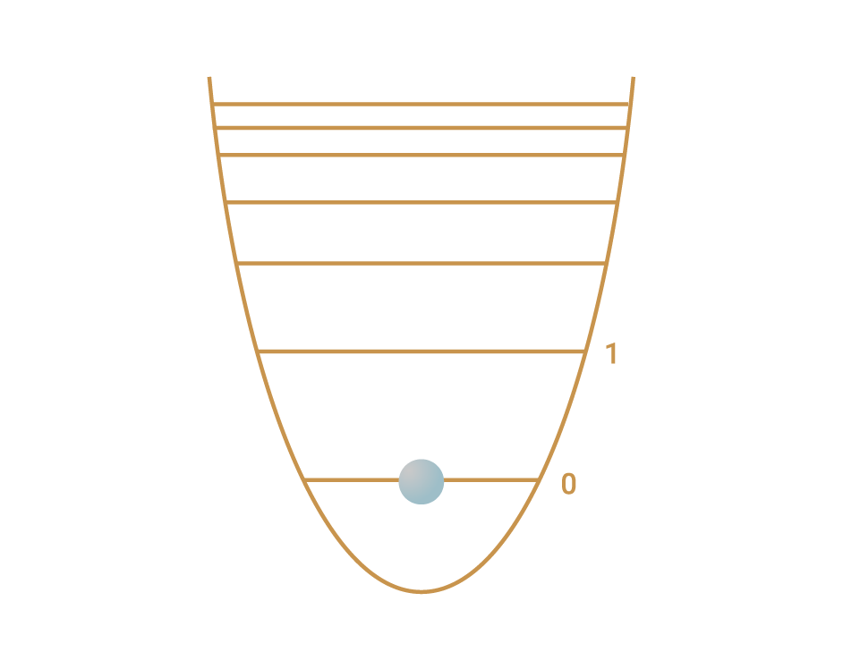
- A qubit is the quantum version of a classical bit and it is encoded in a two-level quantum system.
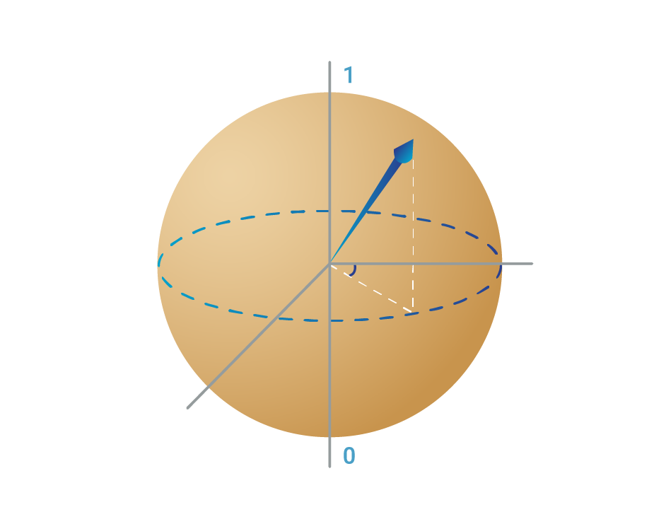
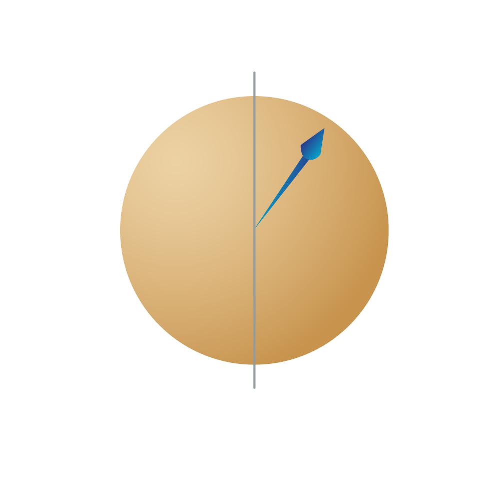
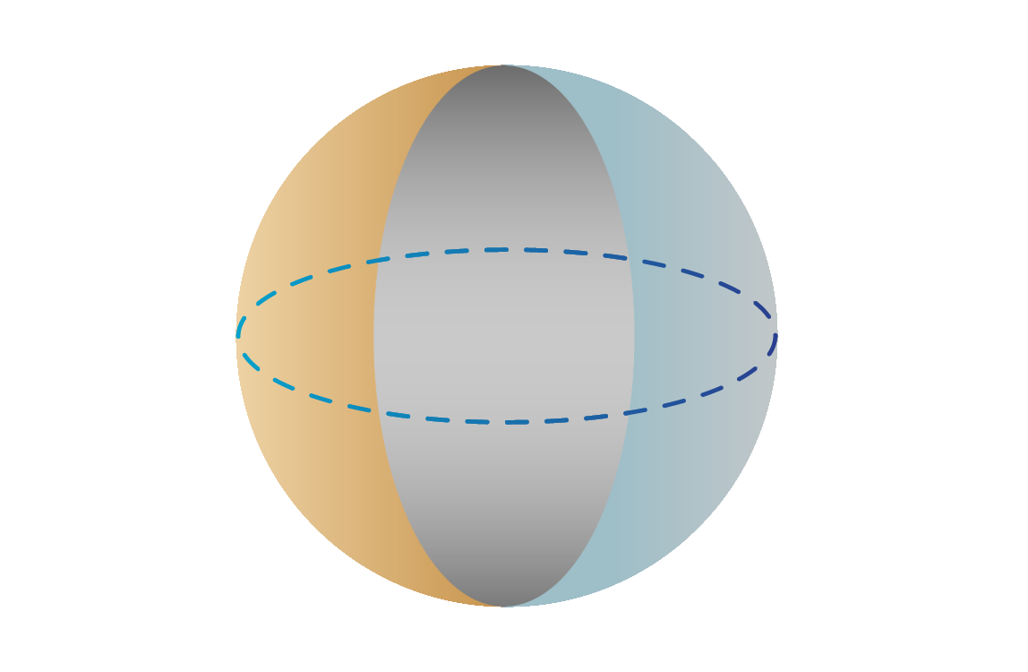
- The high and low energy states represent one and zero. A qubit is often shown with a Bloch sphere representation.
- A qubit’s 1 and 0 have the possibility of existing in a superposition. The qubit can also carry phase information.
- These features are key in quantum computing because they create both new ways of storing information and of processing it. Entanglement is often cited too: this is a superposition spread across the states of two or more qubits.
- To understand how qubits can be realised in different physical systems, check the qubit intros below.
Superconducting
Neutral atom
Neutral atom qubits are encoded in two energy levels of an atom. As all atoms of a given species are identical by nature, the qubits are also identical and do not required sophisticated fabrication procedures.
Solid state qubits
Solid state qubits exploit the inherent quantum nature of particles (e.g. atoms, electrons) in solids by engineering controls to isolate, manipulate and read-out the qubits.
Trapped ions
Trapped ions are charged atoms that are confined in a space using electromagnetic fields.
Photons
Photons hardly interact with each other. This makes them suitable as long-lived flying qubits in quantum computing.
NV centres
Nitrogen-Vacancy (NV) centres consist of a nitrogen atom that has replaced a carbon atom in a diamond lattice and an adjacent vacancy.
The computing paradigms
Gate based – a universal computer that can run any programme written as a series of logic gate operations.
Analogue – annealing finds an energy minimum, solving problems that can be converted into an energy minimisation task.
Measurement-based – a one-way computer that takes a large entangled state as the input.
The challenge
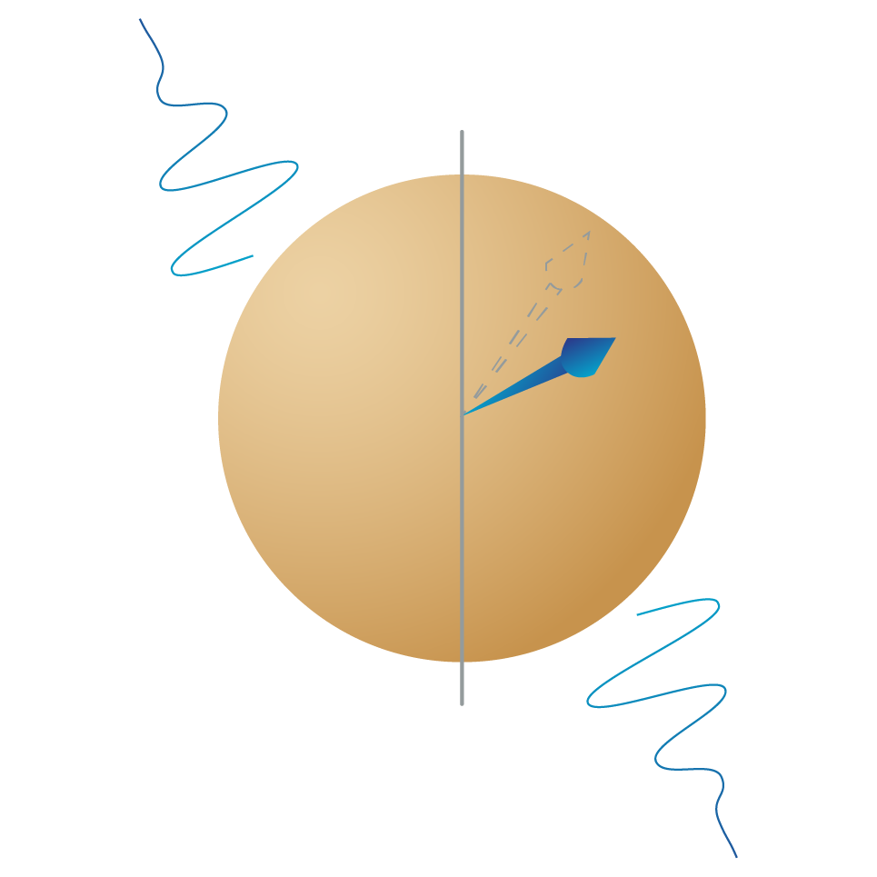
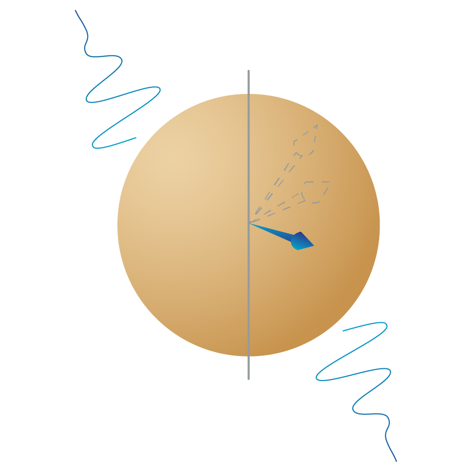
- To protect the quantum state from outside influences that change it, introducing ‘noise’ or errors in your computation.
- To operate on the quantum states to process information, using outside influences to control the qubits’ interactions.
Elementary gates
Gates are the building blocks for algorithms you run on the quantum computer:
- To operate on one qubit to change state or phase.
- To operate on multiple qubits.
Some examples that together are universal (meaning that together they can perform any operations):
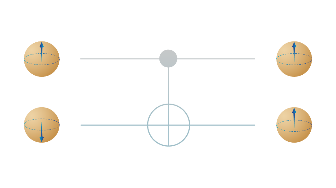
- CNOT – control not, flip the target qubit based on the state of the control qubit.
- Single qubit gates – Pauli X, Y, Z
Types of errors
The baseline metrics
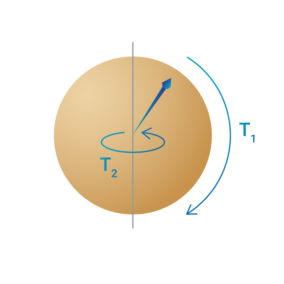
- T1 = how quickly a one changes to a zero.
- T2 = how quickly phase information decays.
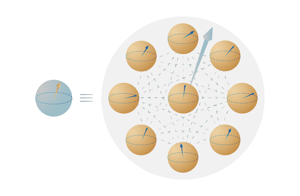
The error-corrected future
- Error correction is a technique to extend the effective coherence time of qubits.
- One ‘logical qubit’ is created from many physical qubits with a code operating on them to erase errors as they arise. The logical qubit has a longer effective coherence time than the individual physical qubits.
- Different error correcting codes exist.
- Error mitigation measures may also help reduce noise.
Beyond counting qubits
- Counting qubits is not enough to tell you the power of your quantum computer because of the impact of noise.
- Quantum volume considers both qubit count and coherence times, multiplying the number of qubits by the achievable circuit depth.
- More useful is the count of logical qubits, meaning the number of error-corrected qubits you create from your physical qubits. The largest number of logical qubits reported so far is 48.
- Another measure is algorithmic qubits. This tells you, for a specific algorithm and noisiness, how many logical qubits you can use for computation. It takes into account whether the algorithm will return an accurate result, known as the result fidelity.
- There are other methods to measure performance too. One approach is randomised benchmarking: this is a test checking if qubits go back to their original state after a cycle of a particular kind of gate called Clifford gates (U†U).
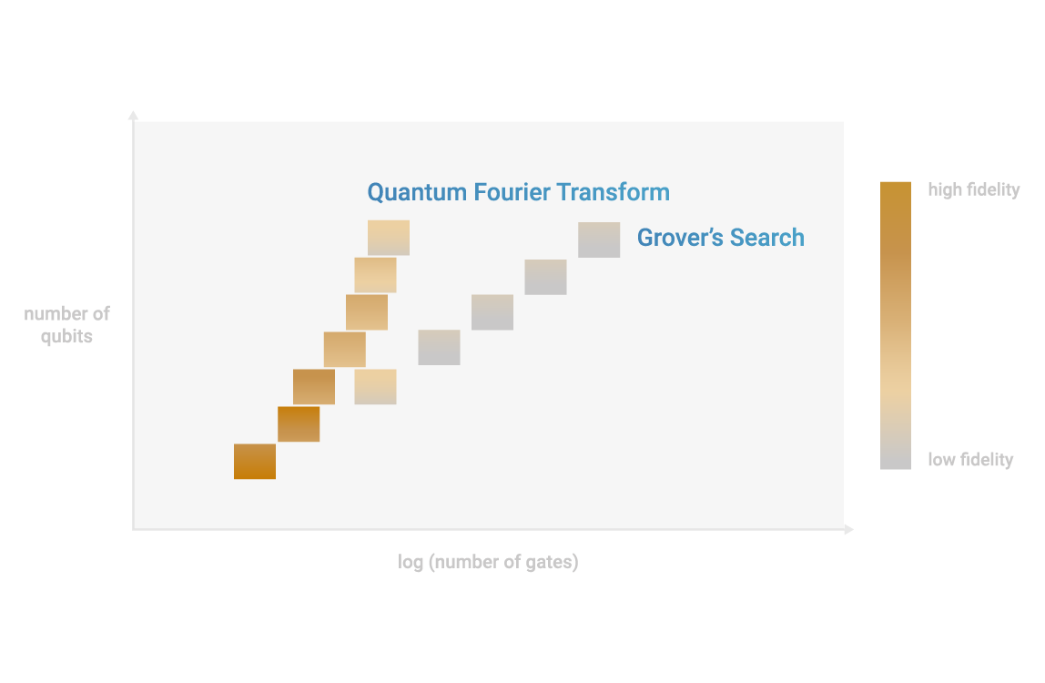
How good an outcome you get from a quantum computation scales differently with the number of qubits for different algorithms. This graphic is adapted from benchmarking work by the Quantum Economic Development Consortium (QED-C).
What algorithms exist?
- Grover
- HHL for linear systems
- Networks of harmonic oscillators
- Quantum Fourier Transform
More algorithms are listed at quantumalgorithmzoo.org
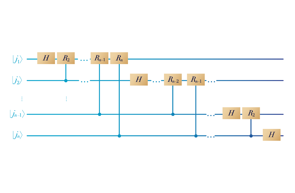
This is a circuit representation of a Quantum Fourier Transform.
Making algorithms efficient
- Qubit encoding schemes can make more efficient use of a limited number of qubits.
- Algorithms operate on data encoded in quantum states. The encoding of data is also known as the QRAM problem.
- We can explore encodings that allow us to pack more information into a single qubit.
- Encoding can make more efficient use of physical hardware.
- Options might include encodings in the quadrants of a Bloch sphere, or in correlations among groups of qubits.
What else to know

- A challenge for practical quantum computing is how to get data into the system. You have to initialise the machine by converting classical data into quantum states.
- Quantum computing is not the solution to all problems. Known algorithms so far can offer improvements for a limited, albeit important, set of calculations.
- The design of quantum memory is still a work in progress.
- Quantum algorithms are often probabilistic, meaning you’ll need to run them multiple times to find the best answer.
- Quantum simulation is something different: it doesn’t necessarily use gates or need error correcting codes, instead arranging qubits to mimic the system of interest, such as a material or network.
- Quantum computers may be used together with digital computers as ‘accelerators’ for certain types of calculation. These setups are described as hybrid.